Nothing quite matches the delight of finding a 100x speedup in an optimization problem. Since my first year of grad school, I’ve been astounded by how small tweaks can produce huge performance differences. This post explores two main approaches to making linear programming problems faster: simplifying the problem formulation, and using warm start. Making the right decisions can result in a 1000x speedup, opening up new research and product options- for instance, making it possible to provide a customer with an instant in-browser or on-device solution, rather than having a delayed offline response.
Code for this study is on Github here
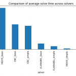
The results: Average solution times (seconds) for solving a 35,000 row optimization problem
| First solve / no warm start (s) | Solution with warm-start (s) | |
| CBC/CLP with for-loop | 73.835 | 2.165 |
| HiGHS with for-loop | 70.922 | 3.535 |
| Clarabel with for-loop | 64.621 | 0.72 |
| HiGHs with transition matrix | 3.622 | 5.149 |
| CBC/CLP with transition matrix | 4.853 | 3.072 |
| CBC/CLP with vector constraint | 4.168 | 2.907 |
| Clarabel with transition matrix | 1.617 | 0.705 |
| Clarabel with vector constraint | 1.568 | 0.365 |
| HiGHS with vector constraint | 0.368 | 0.091 |
| CyLP with custom warm-start | 0.514 | 0.062 |
Background
For this problem, I’m using a problem close to my heart: home battery optimization with separate import costs $p_{\text{buy}}$ and export feed-in-tariff $p_{\text{buy}}$. This is nice simple problem that is interpretable, practical, and has some inherent scaling problems – it’s usually helpful to solve for a full year at a time for system design, but that can be computationally hard depending on your implementation. For more detail, check out the excellent Energy Optimization CE295 course which explores this in the Chapter 5 notes (I’m a former TA for this course).
\(\begin{align}
\min_{\substack{
P_{\text{batt,charge}},\,P_{\text{batt,discharge}},\\
P_{\text{grid,buy}},\,P_{\text{grid,sell}},\,E
}}
\quad &
{p_{\text{buy}}}^T P_{\text{grid,buy},t}
+
{p_{\text{sell}}}^T P_{\text{grid,sell},t}
\\[1em]
\text{s.t.} \quad
& -P^{\max}_{\text{batt}} \le P_{\text{batt,charge}} \le 0 \\
& 0 \le P_{\text{batt,discharge}} \le P^{\max}_{\text{batt}} \\
& 0 \le P_{\text{grid,buy}} \\
& P_{\text{grid,sell}} \le 0 \\
& E^{\min} \le E_t \le E^{\max} \\
& E_{t+1} = E_t
\, – \, \big(
\eta \, P_{\text{batt,charge},t} \,
+
\frac{1}{\eta}P_{\text{batt,discharge},t}
\big) \, \Delta t
\\
& L = P_{\text{batt,charge}}
+ P_{\text{batt,discharge}}
+ P_{\text{grid,buy}}
+ P_{\text{grid,sell}} \\
& E_0 = E^{\min}
\end{align}
\)
We’ll be using the CVXPy optimization package, which provides a simple Pythonic framework for creating describing the variables, constraints, and objectives of a convex optimization problem, and then interface to a variety of modern solvers. Other packages like Pyomo and CVXOpt offer similar functionality. For this, I’m considering three common solvers oriented toward Linear Proramming: Clarabel (the default solver for CVXPy when solving LPs), CBC/CLP from Coin-OR, and the more recent HiGHS. For the custom CLP warm-start, I’ll be using the CyLP package to more directly access the CLP solver (under the hood, CVXPy uses CyLP to interface with the CBC/CLP solver).
As a reference dataset, it’s important to get a realistic sample of the type of heterogeneous data we’d expect in practice: constraint changes which move a previous feasible solution deep into infeasible territory can reduce warm-start benefits. To get realistic meter data, I’m using the Smart Grid, Smart City Australian home energy meter data, and selecting 100 sites which have a full year of uninterruped data from October 2012 through September 2013 (the earliest 12-month period for which full data was available). I use PVGIS to add solar generation sized for a 70% offset of the site’s gross annual load.
All results are shown for a one-shot optimization of one year of data at a 30-minute timestep (17520 timesteps total).
Energy Transition matrix Formulation
A key question is how to implement the energy continuity constraint $E_{t+1} = E_{t} + \ldots$ constraint, where there are three main options:
- Use a for-loop over each timestep, creating a new constraint for each problem. This has a such a large initial solution overhead (>60s) that results are shown in the table but are not plotted. However, once the solver has factorized the problem matrix and saved a useful solution, subsequent warm-start solves can be quite performant!
- Using a state transition matrix: Creating a transition matrix $A = [I \quad 0] \in \mathbb{R}^{N \times N+1}$ allows us to express the problem like $E_{t \in 1 \ldots N} = A^T E + \eta \, P_{\text{batt,charge}} \frac{1}{\eta}P_{\text{batt,discharge}}$. Using sparse matrices, this can be quite efficient.
- Using a simplified vector constraint: Using array slicing to state this as
E[1:] = E[:n] + ...actually is a remarkaby simple hack which works well across a variety of solvers.
Warm-start
Because the optimization surface is flat and the optimum must lie at a vertex of the constraint polytope, linear programming solvers operate via pivot methods, moving between basic feasible solutions. This approach means that we can see a big speedup through using a previously feasible solution a basis to the problem polytope. In practice, this can be accomplished by:
- Saving a feasible solution (some speedup)
- Saving the final problem matrix and solution (more speedup)
- Saving the problem object including basis of the solved problem (most speedup).
However, support for this is not implemented evenly across solvers or within CVXPy. CVXPy typically formulates a problem’s constraint vectors and problem matrices, then passes them down to a lower-level solver interface, which may not support using previous solution information. Simply passing problem.solve(warmstart=True) doesn’t provide any guarantee that you’ll see a performance improvement! It may just reduce the CVXPy overhead in formulating the problem, without reducing the actual solver call time.
A more robust approach is to actually work with the solver interface to tweak the individual problem components: for the CBC/CLP solver this can be done in python via CyLP, or for HiGHS it is done via highspy. Unfortunately, the documentation on this middleware is abysmal and the support teams are tiny.
Expect that the time savings may vary dramatically depending on the type of changes you are making: a change to the objective function without changing constraints can easily net a 100x warm-start speedup (the previous solution is guaranteed to be feasible), while changing large constraints may make the previous solution infeasible and require more solution steps.
Given my experience working with CyLP on a variety of problems, I chose to work with CyLP to develop a custom interface for warm-starting these battery problems.
Results
In the plots below, the “base” columns refer to the transition-matrix constraint approach, and the “simple” solutions refer to the array slicing approach. As mentioned, the for-loop approach is excluded from the plots due to the 10x higher initial solve time.
It’s remarkable that the HiGHS solver has both the worst time (when using the transition-matrix approach), and one of the best times (when using the array-slicing approach). This highlights the need to be creative when formulating a problem. The choice of Clarabel as a default solver seems to be a good one: its performance is relatively invariant to the constraint structure.
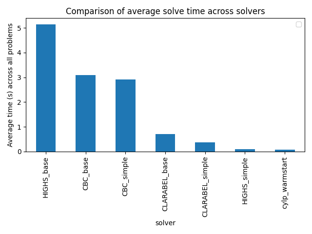
Separating out the solution time for the initial solution from the average time for the subsequent 99 solutions, we see that solvers vary dramatically in their ability to utilize warm start. It appears that the transition-matrix approach prevents HiGHS from taking advantage of any warm-start ability.
And while our CyLP custom warm-start has a higher initial solve time than the HiGHS implementation, on subsequent solves our CyLP warm-start time is 30% lower than the HiGHS warm-start time (0.062s vs 0.091s)!
Conclusion
Warm-start in linear programming is an unappreciated technique for creating orders-of-magnitude speedups in problem solution time. However, careful problem formulation is needed to be able to take full advantage of these benefits, and it may be most effective to work with lower-level interfaces like highspy or CyLP rather than with a high-level wrapper like CVXPy.